Software Performance Benchmarking

In software engineering, “fast” is a subjective term; “throughput of 10,000 operations per second” is an objective fact. However, deriving that fact requires more than just running a timer around a function. It requires a scientific approach to benchmarking that accounts for compiler optimizations, garbage collection, and system stability.

Based on recent comprehensive notes on automated software engineering, I have synthesized a guide on how to approach performance evaluation rigorously—moving from theoretical models to micro-level code analysis and macro-level system profiling.

---

1. The Physics of Throughput: A Theoretical Model

Before we write code to measure performance, we must understand the fundamental behavior of a system under load. We can model a software system as a processor of incoming requests.

The Stable State

To measure anything reliably, a system must be in a stable state. This occurs when the number of requests currently being processed remains approximately constant over time. In this state, the Arrival Rate lambda equals the Throughput X.

• Arrival Rate lambda: The number of requests arriving per unit of time (e.g., requests/sec).
• Throughput X: The number of requests successfully served per unit of time.

If lambda > X, requests arrive faster than they can be served. Queues fill up, latency spikes, and stability is lost.

The Load Diagram: Ideal vs. Real

When we visualize performance, we plot Throughput (X) against the Arrival Rate (lambda).

1. Ideal Behavior: Throughput increases linearly with the arrival rate lambda = X until the system hits its physical limit, known as Maximum Throughput X_max. At this point, Utilization (U) is 100%, calculated as U = X/X_max.
2. Real-World Behavior: Systems rarely hit a hard flat ceiling. Instead, as they approach saturation, overhead (context switching, resource contention) causes throughput to degrade before hitting the theoretical maximum.
3. Thrashing: In severe cases, pushing lambda far beyond X_max causes throughput to actually decrease. This is often due to the system spending more time managing the backlog (e.g., GC thrashing, lock contention) than doing useful work.

---

2. Micro-Benchmarking: The Microscope

Micro-benchmarking involves measuring the performance of small, isolated code fragments. While this sounds simple, it is notoriously difficult in managed environments like the Java Virtual Machine (JVM). As Donald Knuth famously warned, "premature optimization is the root of all evil," but when we do need to optimize critical paths, we must measure accurately.

“premature optimization is the root of all evil” (attributed to Donald Knuth) refers to the danger of spending excessive effort optimizing code before it is even functional or before you know where the actual bottlenecks are

The Pitfalls of Managed Runtimes

In environments like the JVM or .NET, the path from source code to execution is non-linear. If you simply wrap System.nanoTime() around a loop, your results will likely be fundamentally flawed due to the following complex factors:

1. The “Cold Start”: Class Loading & Interpretation

When a process first launches, it is in a “cold” state. Before your logic can even execute, the runtime must perform several heavy-duty tasks:

• Class Loading & Verification: The runtime must locate bytecode files, load them into memory, and verify their structural integrity. This involves significant I/O and CPU overhead.
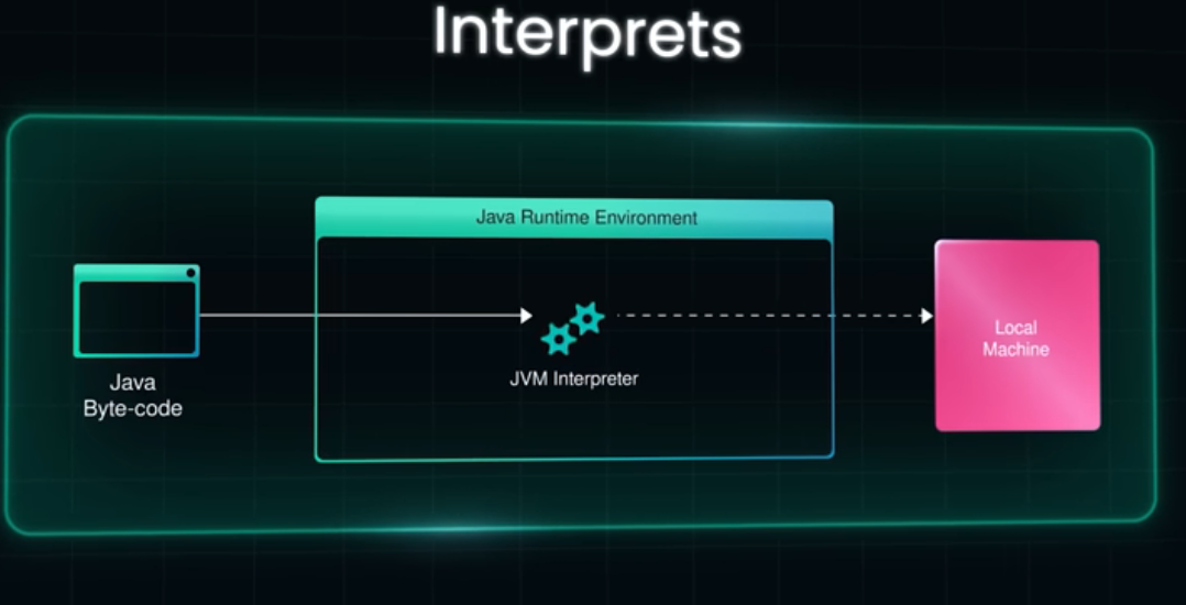
• Interpretation: Initially, the JVM does not run “fast” native code. It uses an interpreter to read bytecode line-by-line. Measuring this phase tells you how fast the interpreter is, not how efficient your algorithm is.

• Resulting Error: If your benchmark doesn’t account for this, your data will be skewed by the high latency of the startup sequence.

  

2. JIT Optimization & The Warmup Phase

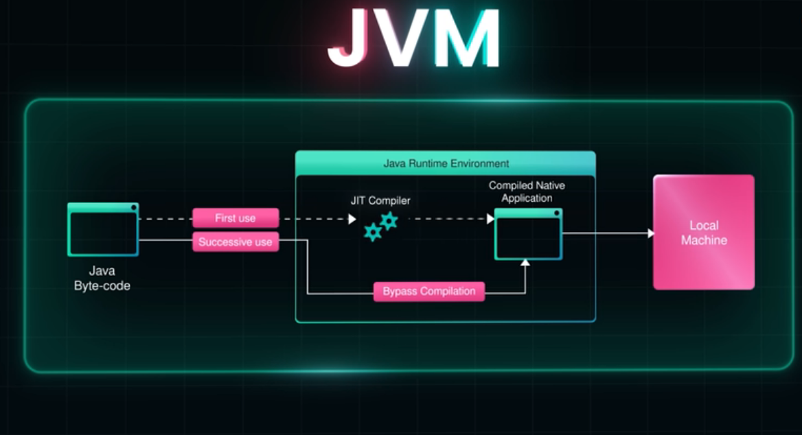
Just-In-Time (JIT) compiler is a dynamic engine that optimizes code based on execution profiles.

• Threshold-Based Compilation: The JIT waits until a method has been called thousands of times (the “invocation threshold”) before it compiles it into native machine code.
• Tiered Compilation: Modern runtimes use multiple levels of optimization. Code might be compiled “simply” at first, and then re-compiled with aggressive optimizations (like method inlining) only after it proves to be a "hotspot".

• Steady-State Requirement: Reliability in benchmarking is only achieved once the code reaches a “stable state” or peak performance. Without a dedicated Warmup Phase—executing the code for several thousand iterations before starting the clock—you are measuring a moving target.

  

  See the video about JIT: The JVM Secret that makes code faster https://www.youtube.com/watch?v=-QHsVHziSZQ&t=135s

3. Dead Code Elimination (DCE) & Constant Folding

The JIT is designed to make production code fast by removing unnecessary work, which can “break” a benchmark.

• DCE Logic: If the compiler determines that the result of a calculation is never used (e.g., it’s not returned, printed, or stored in a global variable), it may delete the entire block of code.
• Constant Folding: If you pass the same hard-coded values into a function every time, the JIT might pre-calculate the result once and simply return that constant value for every subsequent loop iteration.
• The “Zero-Time” Mirage: A developer might see a “0ms” result and think their code is lightning-fast, when in reality, the compiler realized the code was “dead” and didn’t run it at all.

4. Non-Deterministic Background Tasks: Garbage Collection (GC)

Managed runtimes handle memory for you, but this luxury comes at a cost to timing precision.

• Stop-the-World Pauses: The Garbage Collector may trigger a "stop-the-world" (STW) event to reclaim memory at any time. If a GC cycle occurs exactly while your timer is running, your results will show a massive, artificial spike in latency.
• Heuristic Noise: Because you cannot easily predict when a GC will occur, a single-run benchmark is statistically meaningless. You must run enough iterations to either account for or isolate these pauses.

5. De-optimization and Profile Pollution

The JIT makes “optimistic” assumptions. For example, if it sees you only ever pass one type of object into a method, it generates code optimized specifically for that type.

• The Trap: If your benchmark suddenly introduces a different object type halfway through, the JIT must de-optimize, throw away the fast native code, and revert to the slow interpreter to figure out the new logic. This “profile pollution” can make a fast algorithm look slow simply because the environment had to reset itself.

The Solution: JMH (Java Microbenchmark Harness)

To avoid these errors, we use specialized frameworks like JMH. JMH handles the boilerplate of warmup iterations and thread management to ensure we measure peak performance.

Strategies for Accurate Micro-benchmarks

• Use Blackholes: To prevent Dead Code Elimination, we pass results into a "Blackhole" object. This tricks the compiler into thinking the result is needed, forcing the computation to occur.

    @Benchmark
    public void measureRuntime(Blackhole bh) { 
    // The Blackhole forces the JIT to actually execute the constructor
    bh.consume(new NewDataStructure(20, false, 1)); 
    }
  

• Isolate Garbage Collection: GC pauses introduce noise. To measure memory requirements, we can perform separate runs where we incrementally lower the heap size (-Xmx) until the application crashes to find the baseline requirement.
• Parameterization: Run benchmarks against multiple data sizes (e.g., varying payload sizes for a cryptographic check) to see how the algorithm scales.

Hypothetical Example: Benchmarking a Crypto Signature

Instead of a simple loop, a proper JMH test for a signature verification might look like this (conceptually):

@Benchmark
@BenchmarkMode(Mode.Throughput)
@Warmup(iterations = 5) // Handle JVM Warmup
public void testSignature(Blackhole bh) {
    // Consume result to prevent Dead Code Elimination
    bh.consume(myCryptoService.verify(payload));
}

---

3. Macro-Benchmarking: The Landscape

While micro-benchmarks test a single function, Macro-benchmarking evaluates the entire application to identify system-wide bottlenecks.

Profiling Techniques

When the whole system is slow, we use profilers (like VisualVM) to look inside the running process. There are two primary ways to gather data:

1. Sampling: The profiler periodically checks the stack traces of running threads and makes snapshots.
   • Pros: Low overhead, realistic distribution of runtime.
   • Cons: Statistical approximation; might miss very fast, frequent function calls.
2. Profiling: The profiler modifies the bytecode to record every single method entry and exit.
   • Pros: Exact invocation counts.
   • Cons: Changes the original code. Huge performance penalty, potentially distorting the results so much that they no longer reflect reality.

Transient Bottlenecks

Averages lie. A system might show 75% average CPU utilization, but in reality, it could be oscillating between 0% and 100%. These transient bottlenecks (lasting <100ms) can cause massive latency spikes that average metrics completely hide.

---

4. Designing a Benchmark Suite

Whether you are testing a graph database like the LDBC benchmark 25 or a simple web service, a good benchmark must adhere to four criteria:

1. Relevant: It must use realistic data and query patterns.
2. Independent: The test should not be tied to the internal mechanics of one specific implementation.
3. Scalable: The workload should be adjustable from small to massive datasets.
4. Reproducible: The environment (hardware, software, configuration) must be documented so others can verify the results.

---

5. Reporting Your Findings

Finally, data without context is useless. A professional evaluation report should be structured scientifically:

• Research Questions (RQs): Frame the evaluation around specific inquiries (e.g., “How does throughput scale as model size increases?”) rather than simple yes/no questions.
• Visualizations: Use cumulative score plots or runtime bar charts to clearly compare different configurations.
• Threats to Validity: Be honest about the limitations.
  • Internal: Did the measurement tools influence the result?
  • External: Do these results apply to other hardware/OS configurations?
  • Construct: Did we measure the right metric (e.g., is latency a good proxy for user satisfaction here)?

Conclusion

Performance is not an accident; it is an engineered outcome. By distinguishing between stable and overloaded states, utilizing tools like JMH for micro-level precision, and employing statistical sampling for macro-level analysis, we can move from guessing why code is slow to knowing exactly how to fix it.

---

Attribution: This post is a synthesis of concepts and technical notes derived from “ASE-PerformanceBenchmark” by the Critical Systems Research Group.