Query Optimization: SQL vs. NoSQL

As engineers, we often treat databases as black boxes: we put data in, we write a query, and we expect data out. But when a query takes 20 seconds instead of 20 milliseconds, that black box becomes a critical bottleneck. The reality is that disk I/O does not improve at the same rate as CPU power (Moore’s Law), making I/O the single most expensive operation in database systems.

In this post, I want to unpack the internal mechanics of query optimization. We will look at how engines like Microsoft SQL Server transform your declarative SQL into physical operations, and contrast that with the race-condition style optimization used in document stores like MongoDB.

Part 1: The Relational Engine (SQL Server)

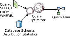
When you submit a SQL query, you aren’t telling the computer how to get the data; you are describing what you want. It is the job of the Query Optimizer to bridge that gap. This process generally follows a specific pipeline: Analyzer → Compiler → Logical Plan → Physical Plan → Execution.

1. The Logical Plan & Relational Algebra

Before the database thinks about disks or indexes, it constructs a Logical Execution Plan. This is a tree of relational algebra operations (Projections, Selections, Joins).

The optimizer’s first goal is to refactor this tree for efficiency without changing the result. A classic technique is Predicate Pushdown.

The Concept:

Imagine joining two massive tables, Users and Orders, but you only care about orders from yesterday. A naive execution might join all 1 million users to all 10 million orders first, and then filter for yesterday. The optimizer “pushes” the date filter down the tree, so it filters the Orders table before the join happens.

Original Scenario:

- The Query
SELECT u.Name, o.Total
FROM Users u
JOIN Orders o ON u.ID = o.UserID
WHERE o.OrderDate = '2023-10-27';

By filtering Orders first, we reduce the input for the join operation drastically.

2. Physical Execution: Join Strategies

Once the logical shape is decided, the engine must choose the physical algorithms to perform the operations. This is cost-based optimization. The engine uses statistics (histograms of data distribution) to estimate the “cost” (mostly I/O) of different methods.

There are three primary join algorithms you must understand:

A. Nested Loop Join

Think of this as a brute-force approach using two for-loops.

# Pseudo-implementation
for user in users_table:       # Outer loop
    for order in orders_table: # Inner loop
        if user.id == order.user_id:
            yield (user, order)

• Use Case: Excellent when one table is very small (e.g., looking up a specific user’s settings). Terrible for large datasets.

B. Hash Join

This is the workhorse for large, unsorted datasets. It works in two phases: Build and Probe.

1. Build: The engine reads the smaller table into memory and builds a Hash Map (key = join column).
2. Probe: It scans the larger table, hashes the join column, and checks the map for matches.

• Use Case: Heavy analytical queries where large tables are joined and no useful index exists on the join keys.

The Scenario

Imagine we are analyzing e-commerce data. We need to join two tables:

1. Customers (Small table: 1,000 rows)

2. Orders (Large table: 1,000,000 rows)

We want to find all orders for customers in a specific region. No indexes exist on the joining columns.

The Algorithm: Two-Phase Execution

The database engine performs this join in two distinct phases.

Phase 1: The Build Phase (In-Memory)

The engine identifies the smaller input (the “Build” input), which is the Customers table. It reads these rows into memory and creates a Hash Table.

• Key: The join column (CustomerID).
• Value: The data we need to select (e.g., CustomerName, Region).

This structure allows for O(1) lookups.

Phase 2: The Probe Phase

Once the hash table is built, the engine begins scanning the larger Orders table (the “Probe” input) row by row.

1. For every order, it takes the CustomerID.
2. It hashes this ID using the same hash function used in Phase.
3. It checks the Hash Table for a match.
   • Match found: The combined row (Customer + Order) is returned.
   • No match: The row is discarded.

C. Sort Merge Join

If both sides of the join are already sorted (perhaps due to an index), the engine can “zip” them together efficiently.

# Pseudo-implementation (assuming sorted inputs)
ptr_u = 0
ptr_o = 0
while ptr_u < len(users) and ptr_o < len(orders):
    if users[ptr_u].id == orders[ptr_o].user_id:
        yield (users[ptr_u], orders[ptr_o])
        ptr_o += 1 # Advance pointer
    elif users[ptr_u].id < orders[ptr_o].user_id:
        ptr_u += 1
    else:
        ptr_o += 1

• Use Case: Extremely fast for large datasets if they are indexed (sorted) on the join key.

3. Access Methods: Scan vs. Seek

How does the database actually retrieve the rows?

• Table Scan: Reading every page of the table. Useful only for very small tables or when you requested >50% of the rows.

  • Example:SQL

      -- Assuming no index exists on 'Comment'
      SELECT  FROM Orders WHERE Comment LIKE '%urgent%';
    

  • The Mechanics: The engine must load all 1,000,000 rows into memory to check the Comment field for the text “urgent”.
  • Performance: Generally the slowest method for specific lookups, but efficient for small tables.

• Index Scan: Reading all leaf nodes of an index.

  An Index Scan is similar to a Table Scan, but instead of reading the heavy table data (the “heap”), the engine reads the leaf nodes of an index. This is lighter because the index usually contains fewer columns than the full table.

  When it happens: Used when the query needs to scan data, but the data required is entirely present in an index (Covering Index), or when sorting is required.

  • Example:

      -- Assuming a Non-Clustered Index exists on (OrderDate)
      SELECT OrderDate, COUNT()
      FROM Orders
      GROUP BY OrderDate;
    

  • The Mechanics: The engine scans the OrderDate index from start to finish. It never touches the actual Orders table data because the date is all it needs. It reads the index leaf pages sequentially.

  ### 3. Index Seek

• Index Seek: The gold standard Navigating the B-Tree structure to find a specific key or range. This is O(log N).

  This is the “sniper” approach and the most efficient method for retrieving specific rows. The engine uses the B-Tree structure of the index to navigate directly to the specific record(s) you asked for.

  • When it happens: Used when you filter by a column that is indexed using operators like =, >, <, or BETWEEN

  • Example:

      -- Assuming a Clustered Index (Primary Key) on OrderID
      SELECT  FROM Orders WHERE OrderID = 54321;
    

  • The Mechanics: Instead of reading row 1, then row 2, etc., the engine starts at the root of the B-Tree. It determines that 54321 is in the right branch, jumps to the next level, and repeats until it hits the specific leaf page containing ID 54321. It typically reads only 3 or 4 pages of data instead of thousands.

Part 2: SQL Best Practices

Understanding the engine internals dictates how we should write SQL. Here are specific patterns to adopt and avoid.

1. Avoid Non-Sargable Queries

“SARGable” stands for Search ARGument able. If you wrap a column in a function within your WHERE clause, the optimizer often cannot use the index, forcing a full table scan.

Bad (Non-Sargable):

-- The engine must apply YEAR() to every single row to check this.
SELECT  FROM Employees WHERE YEAR(HireDate) = 2023;

Good (Sargable):

-- The engine can Seek the index for the range.
SELECT  FROM Employees
WHERE HireDate >= '2023-01-01' AND HireDate < '2024-01-01';

2. The SELECT * Problem

Beyond network overhead, SELECT * can prevent Covering Indexes. If you have an index on (UserID, Email) and you run SELECT Email FROM Users WHERE UserID = 5, the engine can get the answer directly from the index (which is smaller and faster). If you do SELECT *, it must look up the index and then go fetch the rest of the row from the main storage - Clustered Index (Key Lookup), doubling the I/O.

3. Procedural vs. Declarative

SQL is declarative. Avoid trying to force procedural logic (cursors, complex loops) inside the database. The optimizer is smarter than your loop. Also, avoid IN or EXISTS if a standard JOIN can achieve the same result, though modern optimizers handle IN very efficiently now (often rewriting it to a semi-join).

---

Part 3: The NoSQL Paradigm (MongoDB)

Optimization in NoSQL document stores like MongoDB shares goals with SQL (reduce I/O), but the implementation differs significantly because there are no rigid schemas or joins (conventionally).

1. The “Race” Model

While SQL Server uses cost estimation formulas to pick a plan, MongoDB uses an empirical competition model.

1. The query planner identifies all indices that could support the query.
2. It generates candidate plans for each index.
3. It runs these plans in parallel in a race.
4. The first plan to return roughly 101 documents (a specific batch size) wins.
5. The winning plan is cached and used for subsequent queries of the same “shape”.

If a cached plan starts performing poorly (e.g., data distribution changes), the server evicts the cache and re-runs the race.

2. Optimization Steps in the Pipeline

Just like SQL pushes predicates down, MongoDB optimizes aggregation pipelines by moving reducing stages to the front:

• Filter Early: $match stages should be as early as possible.
• Limit Early: $limit and $skip are moved before $project where possible to reduce the volume of data passing through the pipeline.

3. Understanding explain()

To debug MongoDB performance, we use .explain("executionStats"). You must look for the stage types:

• COLLSCAN: Collection Scan. The equivalent of a full Table Scan. usually bad.
• IXSCAN: Index Scan. The engine is using the index keys. Good.
• FETCH: The engine found the key in the index but had to go to the document to get the rest of the data.

Example Scenario:

You have a collection Sensors with millions of documents.

// Query
db.Sensors.find({ region: "EU-West", status: "Active" })

If you only have an index on region, the engine does an IXSCAN to find all “EU-West” docs, then must FETCH every single one to check if the status is “Active”.

Optimization: Create a Compound Index { region: 1, status: 1 }. Now the query can be fully satisfied by the IXSCAN alone.

Summary

Whether you are scaling a relational cluster or a document store, the physics remains the same:

1. I/O is the enemy.
2. Indexes are your primary weapon, but they come with write-cost.
3. Visibility is key. Use Execution Plans (SQL) and Explain (Mongo) to verify your assumptions.

---

Attribution: This blog post is a synthesis of concepts derived from the Query Optimization lecture materials by BME JUT (Automatizálási és Alkalmazott Informatikai Tanszék) and associated readings on SQL Server and MongoDB internals.